Wetland Extent

Wetland extent data was obtained from the Oakland Ridge National Laboratory Distributed Active Archive Centre (Hess et al., 2015). The raster was cropped to along the middle-lower Amazon River and resampled to the inundation frequency (IF) raster’s resolution. The raster contains information on wetland cover during both low-water and high-water stage in the Amazon, but because the IF-depth model is calibrated using survey data collected during the flooding season, the high-water stage wetland data was used to mask the IF data. For detailed code on how the raster was processed using rasterio and rioxarray, please refer to this repository.

import numpy as np
import matplotlib.pyplot as plt
import rasterio as rio
from matplotlib.patches import Patch
from matplotlib.colors import ListedColormap

# Import wetland extent
wetland = rio.open("../data/wetland_nearest.tif")

# Read into a NumPy array (only 1 band)
wetland_np = wetland.read(1)

# Group values into categories
wetland_group = np.zeros_like(wetland_np)  # Initialize grouped array
wetland_group[wetland_np == 1] = 0 # Background
wetland_group[(wetland_np == 11) | (wetland_np == 21) | (wetland_np == 41)| (wetland_np == 51)] = 1  # Open water
wetland_group[(wetland_np == 13) | (wetland_np == 23) | (wetland_np == 33)] = 2  # Macrophyte
wetland_group[(wetland_np == 44) | (wetland_np == 66)] = 3  # Non-flooded shrub/ woodland
wetland_group[(wetland_np == 45) | (wetland_np == 55)] = 4  # Flooded shrub
wetland_group[(wetland_np == 67) | (wetland_np == 77)] = 5  # Flooded woodland
wetland_group[(wetland_np == 88)] = 6  # Non-flooded forest
wetland_group[(wetland_np == 89) | (wetland_np == 99)] = 7  # Flooded forest

# Custome palette
custom_colors = ['#000000','#2559DE', '#E432BF', '#EE8761', '#97EBD9', '#A0C0FF', '#FFFF00', '#59A52F']
cmap = ListedColormap(custom_colors) # Create a discrete colormap

# Custom labels
labels = [
    "",
    "Open water",
    "Macrophyte",
    "Non-flooded shrub/ woodland",
    "Flooded shrub",
    "Flooded woodland",
    "Non-flooded forest",
    "Flooded forest"
]

# Plot
fig, ax = plt.subplots(figsize=(10, 4))
img = ax.imshow(wetland_group, cmap=cmap)

# Set background to beige
fig.patch.set_facecolor("#F9F8F2")
ax.set_facecolor("#F9F8F2")

# Add a discrete legend
legend_patches = [Patch(color=custom_colors[i], label=labels[i]) for i in range(len(labels))]
legend = ax.legend(
    handles=legend_patches,
    loc='lower right',
    bbox_to_anchor=(1.0, 0.05),
    frameon=False, # No frame
    fontsize=8,
    ncol=2,                   # Split into 2 columns
    columnspacing=1.2,        # Space between columns
    labelcolor='white'        # White text
)

# Remove axes for clean aesthetics
ax.axis("off")

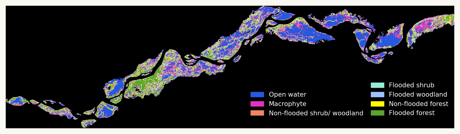
Figure 1: Wetland extent during high-water stage

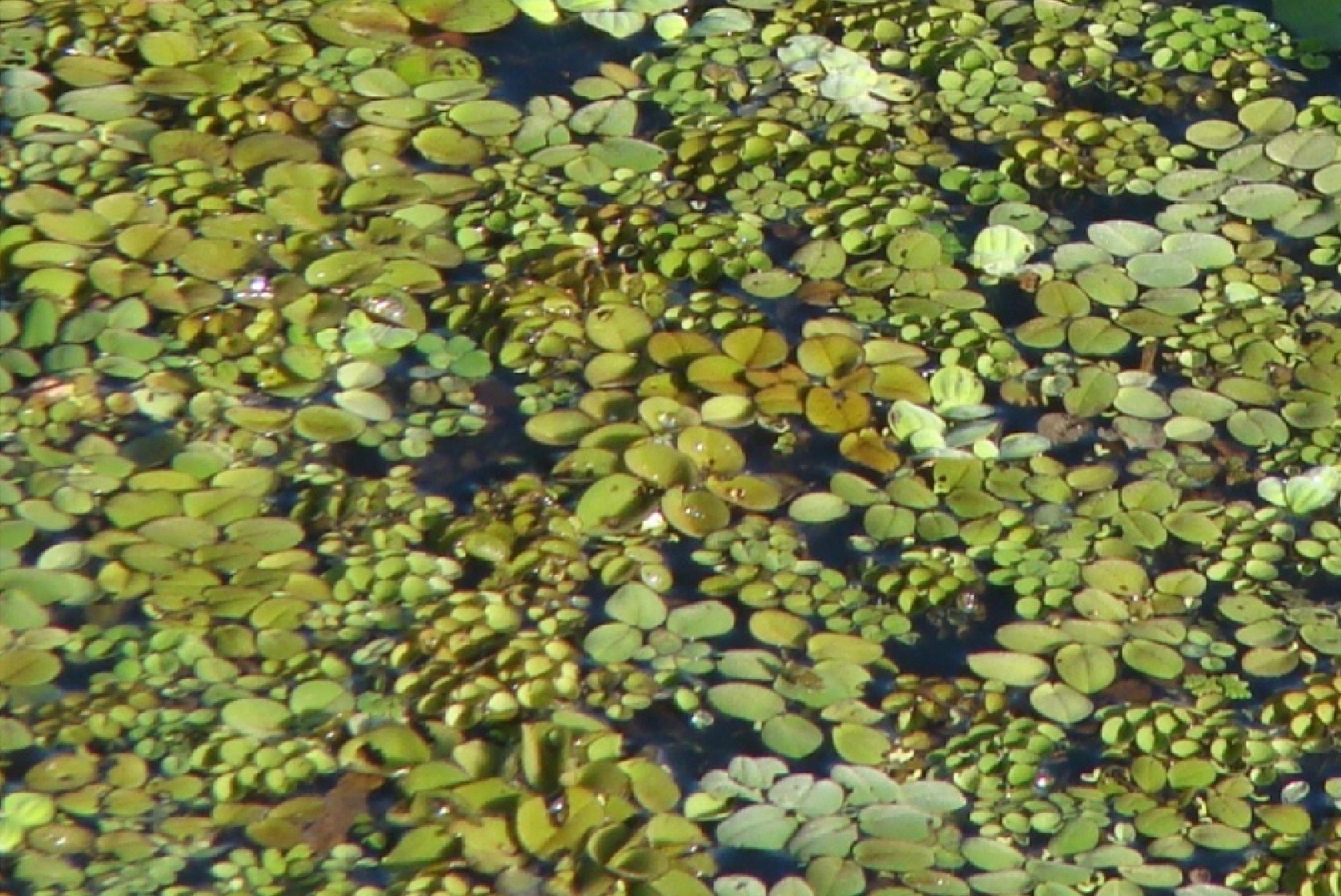
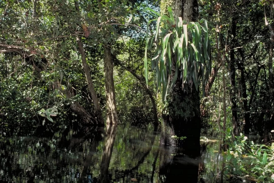
The vegetation cover in the middle-lower Amazon is diverse, ranging from aquatic macrophytes (herbaceous plants) that grow in or near the water, to forests that are annually submerged under water.

Figure 2: Macrophytes (Mortillaro et al., 2016)

Figure 3: Flooded forest (Amazon Waters Alliance, 2024)