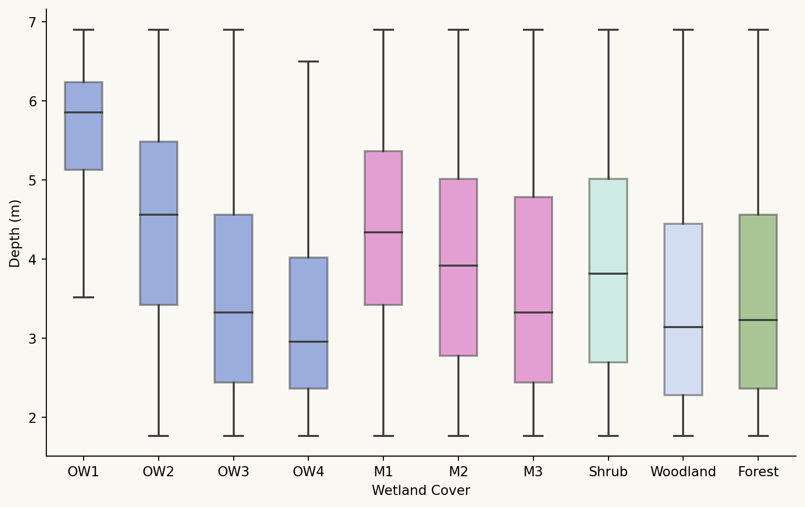
Grouping the bathymetry values by wetland cover and visualizing them as boxplots, an interesting pattern emerges. Wetland cover is defined as open water (OW), macrophytes (M), shrub, woodland, and forest, with the colours in the boxplot corresponding to the colours in the wetland extent map.
Considering the overall average of each group, the depth generally decreases from open water to macrophytes and to flooded forests. This is expected because the forests are found further away from the water bodies than the macrophytes, and macrophytes are adapted to life in water, while the forests are only seasonally inundated.
Code
import numpy as npimport pandas as pdimport matplotlib.pyplot as pltimport rasterio as rioimport seaborn as sns# Import bathymetrybathymetry = rio.open("data/bathymetry.tif")bathymetry_np = bathymetry.read(1) # numpy arraybath_values = bathymetry_np.flatten() # flatten# Import wetland extentwetland = rio.open("data/wetland_nearest.tif")wetland_np = wetland.read(1) # numpy array# Group wetland values into categorieswetland_group = np.zeros_like(wetland_np) # Initialize grouped arraywetland_group[(wetland_np ==0) | (wetland_np ==1)] =0# Backgroundwetland_group[(wetland_np ==11)] =1# Open water Awetland_group[(wetland_np ==21)] =2# Open water B wetland_group[(wetland_np ==41)] =3# Open water C wetland_group[(wetland_np ==51)] =4# Open water Dwetland_group[(wetland_np ==13)] =5# Macrophyte A wetland_group[(wetland_np ==23)] =6# Macrophyte B wetland_group[(wetland_np ==33)] =7# Macrophyte Cwetland_group[(wetland_np ==45)] =8# Shrubwetland_group[(wetland_np ==77)] =9# Woodlandwetland_group[(wetland_np ==88) | (wetland_np ==89) | (wetland_np ==99)] =10# Forest# Flatten the arraywetland_values2 = wetland_group.flatten() # Create dataframe with bathymetry and grouped wetland valuesdf2 = pd.DataFrame({'Bathymetry': bath_values, 'Wetland': wetland_values2})# Exclude rows where the wetland category is 0df_filtered = df2[df2['Wetland'] !=0]# Palettepalette = ['#2559DE', '#2559DE', '#2559DE', '#2559DE', '#E432BF', '#E432BF', '#E432BF', '#97EBD9', '#A0C0FF', '#59A52F']# Labelslabels = ['OW1', 'OW2', 'OW3', 'OW4', 'M1', 'M2', 'M3', 'Shrub', 'Woodland', 'Forest']# Box plot using seabornplt.figure(figsize=(10, 6))sns.boxplot(x='Wetland', y='Bathymetry', data=df_filtered, palette=palette, showfliers=False, # Turn off outliers width=0.5, # Make the boxes narrower fliersize=0, # Ensures that outliers are not shown, even if there are some left linewidth=1.5, # Adjust line width for the boxes boxprops=dict(alpha=0.5)) # Set box transparency# Format graphplt.title("") # Remove default titleplt.suptitle("")plt.xticks(ticks=range(len(labels)), labels=labels, fontsize=10) # Apply custom labelsplt.xlabel("Wetland Cover") # x-axis labelplt.ylabel("Depth (m)") # y-axis labelplt.gca().set_facecolor('#F9F8F2') # Background colorplt.gcf().patch.set_facecolor('#F9F8F2') # Figure background colorplt.gca().spines['top'].set_visible(False) # Turn off top axis lineplt.gca().spines['right'].set_visible(False) # Turn off right axis lineplt.show()
Figure 1: Box plot of bathymetry by wetland cover
Within the open water group and the macrophyte group, bathymetry values vary depending on the vegetation cover of each group at low-water stage. From open water, to non-flooded herbaceous and flooded herbaceous, and to non-flooded shrub and flooded shrub, the average bathymetry decreases clearly, especially for the open water group. As discussed, this trend reflects the natural distribution of vegetation, with shrubs typically located further from the water bodies than herbaceous plants.